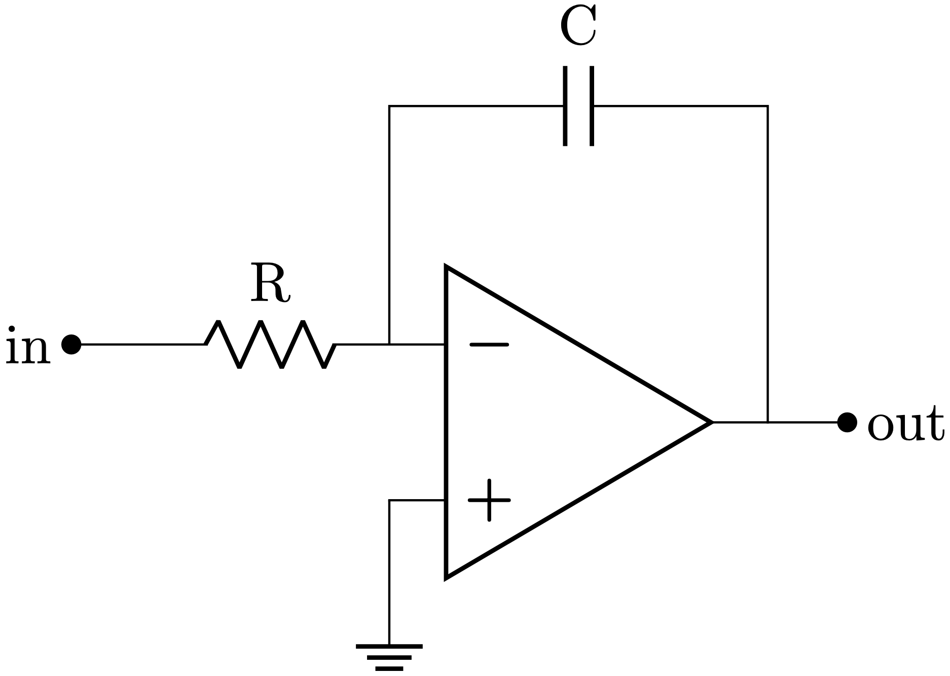
Laplace analysis
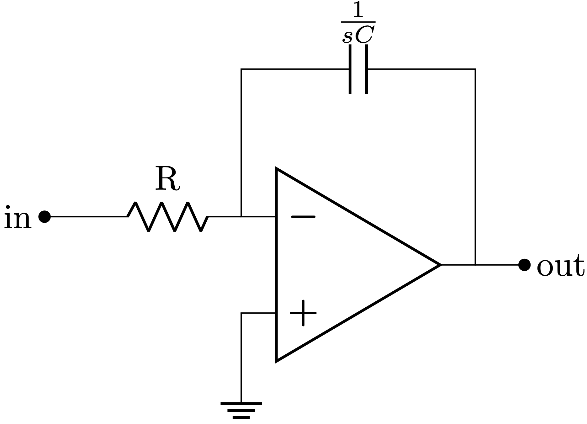
\[H\left(s\right) = – \frac{\frac{1}{sC}}{R} = – \frac{1}{sRC}\]
Bilinear (or Tustin) transform
The Laplace transfer function can be approximated into the Z domain using the bilinear or tustin transform. The mapping between Laplace and Z domain using the first order approximation of the bilinear transform is:
\[s = \frac{2}{T_s} \frac{z-1}{z+1}\]
Replacing \(s\) with previous expression, we can get the following transfer function in the Z domain:
\[H\left( z \right) =H\left(s\right)\bigg|_{s = \frac{2}{T} \frac{z – 1}{z + 1}} = – \frac{1}{\frac{2}{T_s } \frac{z-1}{z+1} RC } = -\frac{z+1}{\frac{2}{T_s} RC \left(z – 1\right)} = -\frac{T_s}{2RC} \frac{z+1}{z-1}\]
The transfer function can now be transformed into a finite differences equation:
\[\frac{Y\left(z\right)}{X\left(z\right)} = -\frac{T_s}{2RC} \frac{z+1}{z-1} = -\frac{T_s}{2RC} \frac{1 + z^{-1}} {1 – z^{-1}}\]
\[Y\left(z\right) \left(1 – z^{-1} \right) = -\frac{T_s}{2RC} \left(1 + z^{-1}\right)\]
\[y[n] – y[n-1] = -\frac{T_s}{2RC} \left(x[n] + x[n-1]\right)\]
\[y[n] = -\frac{T_s}{2RC} \left( x[n] + x[n-1] \right) + y[n-1] \]
Python implementation
from scipy import signal
import numpy as np
import matplotlib.pyplot as plt
# Sampling frequency
fs = 1e4
# Sampling period
Ts = 1/fs
# Amplitude
A = 2.0
# Number of periods to represent
n_periods = 1
# Sine frequency (Hz)
f = 200
# Total time to represent
t_total_time = n_periods * 1/f
# Resistance (Ohms)
R = 1e3
# Capacitance (Farads)
C = 1e-6
def integrate(current_in, prev_in, prev_out):
"""
Perform sample integration on OA integrator circuit
"""
return Ts/(2*R*C) * (current_in + prev_in) + prev_out
# Time array
t = np.arange(0, t_total_time, Ts)
# Sine signal
sine = A * np.sin(2*np.pi*f*t)
# Constant signal
const = A * np.ones(len(t))
# Initialize output arrays to 0
out_sine = np.zeros(len(t))
out_const = np.zeros(len(t))
# Check that length is the same. Otherwise, for loop below
# has to be split
assert(len(out_sine) == len(out_const))
# Pass input signal through integrator (compute output values)
for n in range(1, len(out_sine)):
out_sine[n] = integrate(sine[n], sine[n-1], out_sine[n-1])
out_const[n] = integrate(const[n], const[n-1], out_const[n-1])
# Plot input and output signals
fig = plt.figure()
plt.subplot(211)
plt.plot(t, sine)
plt.title('Input signal (sine)')
plt.ylabel('Amplitude')
plt.xlabel('Time (s)')
plt.grid(True)
plt.subplot(212)
plt.title('Output signal')
plt.plot(t, out_sine)
plt.xlabel('Time (s)')
plt.ylabel('Amplitude')
plt.grid(True)
fig.tight_layout()
plt.savefig('sine_integration.png', dpi=300)
plt.show()
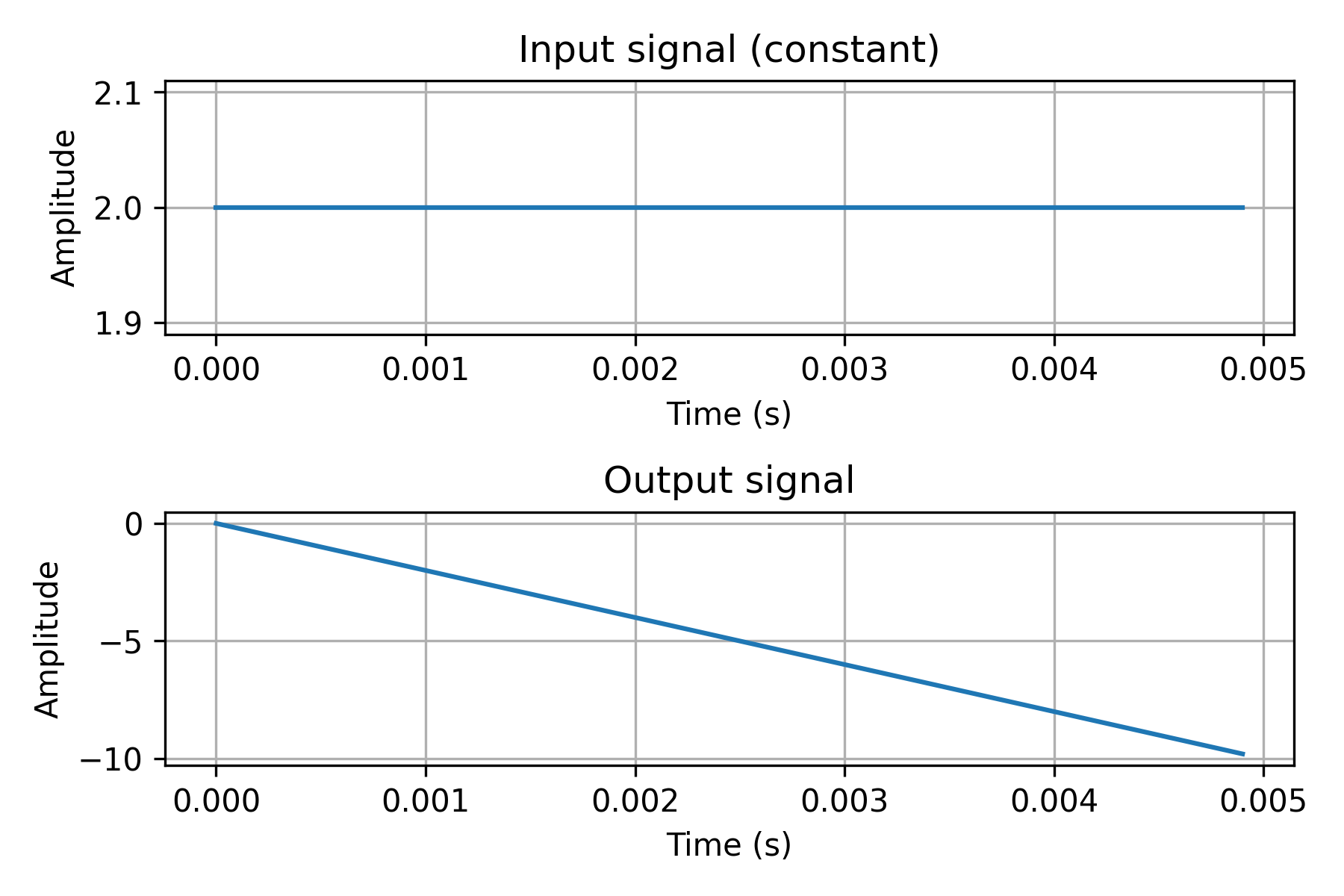
fig = plt.figure()
plt.subplot(211)
plt.plot(t, const)
plt.title('Input signal (constant)')
plt.ylabel('Amplitude')
plt.xlabel('Time (s)')
plt.grid(True)
plt.subplot(212)
plt.title('Output signal')
plt.plot(t, out_const)
plt.xlabel('Time (s)')
plt.ylabel('Amplitude')
plt.grid(True)
fig.tight_layout()
plt.savefig('const_integration.png', dpi=300)
plt.show()

LaTeX code used to generate circuit schematic
\begin{circuitikz} []
	\ctikzset{resistors/scale=0.7, capacitors/scale=0.6}
        \draw (0,0)  node[left]{in} to[short, *-] ++(0.5, 0)  to[R, l=R] ++(1.5,0)  coordinate(inm) node[op amp, anchor=-](OA){};
	\draw (inm) -- ++(0, 1.5)  coordinate(C_left) to[C, l=C] (C_left -| OA.out) -- (OA.out) to[short, -*] ++(0.5, 0) node[right]{out};
	\draw (OA.+) -- ++(0, -0.5) node[ground]{};
\end{circuitikz}

\begin{circuitikz} []
	\ctikzset{resistors/scale=0.7, capacitors/scale=0.6}
        \draw (0,0)  node[left]{in} to[short, *-] ++(0.5, 0)  to[R, l=R] ++(1.5,0)  coordinate(inm) node[op amp, anchor=-](OA){};
	\draw (inm) -- ++(0, 1.5)  coordinate(C_left) to[C, l=$\frac{1}{sC}$] (C_left -| OA.out) -- (OA.out) to[short, -*] ++(0.5, 0) node[right]{out};
	\draw (OA.+) -- ++(0, -0.5) node[ground]{};
\end{circuitikz}