In the following Python script it is shown how the aliasing effect (having signals whose frequency is beyond half of the sampling frequency, i.e., \(\frac{f_s}{2}\)) can be intuitively understood as a folding of the frequencies outside the \(\left[0, \frac{f_s}{2}\right]\) range.

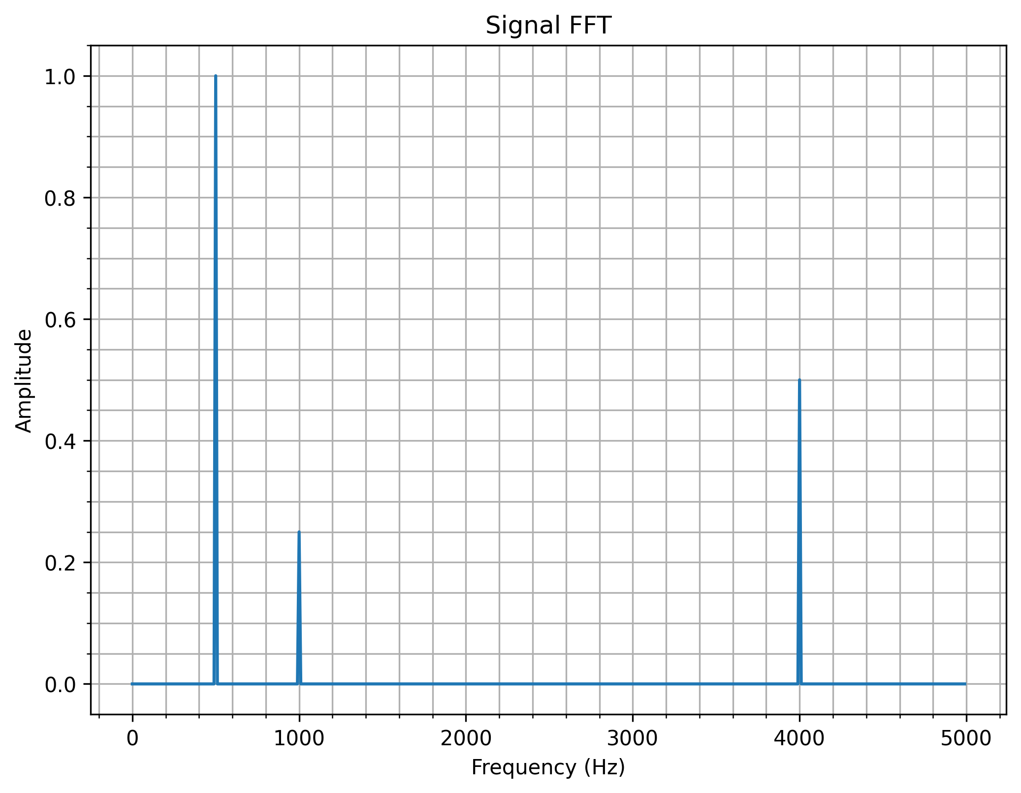
In the script, the sampling frequency is 10 kHz. Then, 3 sinusoids of frequency \(f_{s1} = 500~Hz\), \(f_{s2} = 6~kHz\) and \(f_{s3} = 11~kHz\) are generated. The FFT of the sum of s1, s2 and s3 is computed and plotted. Given that the Nyquist frequency in the system is 5 kHz, it can be seen on the FFT plot how the frequencies wrap around \(\frac{f_s}{2}\) and 0.

Just as a reminder, the way the X-axis on the FFT is explained in FFT resolution.

import numpy as np
import numpy.fft as fft
import matplotlib.pyplot as plt

# Define sampling frequency 
fs = 10e3
Ts = 1/fs

# Define time array
n_periods = 1000
total_time = 1/fs * n_periods
t = np.arange(0, total_time, Ts)


# %% Define signal 1
f1 = 500
s1 = np.sin(2*np.pi*f1*t)


# %% Define signal 2
# Since fs = 5_000, f2 will fold to 4_000 Hz bin
f2 = 6_000
s2 = 0.5 * np.sin(2*np.pi*f2*t)

# %% Define signal 3
# Since fs = 5_000, f3 will fold first on 5_000 Hz and then on 0 again. Therefore, f3 will be shown at 1_000 Hz bin
f3 = 11_000
s3 = 0.25 * np.sin(2*np.pi*f3*t)

# %% Define signal as a sum of s1, s2 and s3
s = s1 + s2 + s3

# %% Compute FFT 
# Total number of samples 
N_samples = len(s)
print(f"Number of samples: {N_samples}")
# Floor in case division is not integer
half_N_samples = int(np.floor(N_samples/2))
# Define frequency bin width 
delta_f = fs/N_samples

# Compute frequency bins until Nyquist frequency
freq_bins = np.arange(0, fs/2, delta_f)

Y = fft.fft(s)

plt.figure(figsize=(8,6), dpi=300)

# Plot only half of the FFT result. Plot absolute value and scale it to represent amplitude
plt.plot(freq_bins, 2.0 / N_samples * np.abs(Y)[:half_N_samples])
plt.grid(True, which='both')
plt.minorticks_on()
plt.title('Signal FFT')
plt.xlabel('Frequency (Hz)')
plt.ylabel('Amplitude')
plt.show()

DFT can be thought as a simple change of basis. In the time domain, every sample of a signal represents its amplitude at that very instant.

\[ y\left[n\right] = \sin{\left( \frac{2\pi k }{N} n\right)} \]

\[ k = 2, N = 64\]

Nevertheless, when applying a transformation such as the DFT, every sample means something different.

The DFT is computed as the scalar product between the signal and a orthogonal base. This base is as follows:

\[ \{\boldsymbol{w}^{(k)}\}_{\{k=0,1,…,N-1\}} \]

\[ w_n = e^{j \frac{2\pi}{N}nk}\]

If some of these base vectors are plotted with the imaginary part in the Y axe and the real part in the X axe:

Real and imaginary part of the DFT basis with N=64

DFT calculation

The DFT of a signal can be computed then, applying a change of basis over the desired signal.

\[ X\left[k\right] = \sum_{n=0}^{N-1} x\left[n\right] e^{-j\frac{2\pi}{N}nk}, \text{      } k = 0,1,…,N-1 \]

DFT of a \(\delta\left[n\right]\)

\[ x\left[n\right] = \delta[n] = \left\{\begin{matrix}
1 & n = 0\\
0 & otherwise
\end{matrix}\right. \] \[X\left[k\right] = \sum_{n=0}^{N-1}{\delta\left[n\right] e^{-j\frac{2\pi}{N}nk}}\]

\[ X\left[k\right] =  1 \cdot e^{-j\frac{2\pi}{N}\cdot 0 \cdot k} = 1 \]

DFT of a cosine

\[ x\left[n\right] = 4 \cos{\left(\frac{2\pi}{4}n\right)} =  4 \cos{\left(\frac{2\pi 4}{16}n\right)} = \frac{4}{2} \left[e^{ \frac{2\pi}{16} 4n} + e^{-j \frac{2\pi}{16} 4n} \right]\]

[To be finished]
 

A vector space basis is the skeleton from which a vector space is built. It allows to decompose any signal into a linear combination of simple building blocks, namely, the basis vectors. The Fourier Transform is just a change of basis.

A vector basis is the linear combination of a set of vector that can write any vector of the space.

\[ w^{(k)} \leftarrow \text{basis} \]

The canonical basis in \(\mathbb{R}^2\) are:

\(e^{(0)} = [1, 0]^T \ \ e^{(1) } = [0,1]^T \)

Nevertheless, there are more basis for \(\mathbb{R}^2\):

\(e^{(0)} = [1, 0]^T \ \ e^{(1) } = [1,1]^T \)

This former basis is not linearly independent as information of \(e^{(0)}\) is inside \(e^{(1)}\).

Formal definition

H is a vector space.

W is a set of vectors from H such that \(W = \left\{ w^{(k)}  \right\} \)

W is a basis of H if:

  1. We can write \( \forall x \in H\): \( x = \sum_{k=0}^{K-1} \alpha_k w^{(k)}, \ \ \alpha_k \in \mathbb{C} \)
  2. \( \alpha_k  \) are unique, namely, there is linear independence in the basis, as a given point can only be expressed in a unique combination of the basis.

Orthogonal basis are those which inner product returns 0:

\( \left \langle w^{(k)}, w^{(n)} \right \rangle = 0, \ \ \text{for } k \neq n \)

In addition, if the self inner product of every basis element return 1, the basis are orthonormal.

How to change the basis?

An element in the vector space can be represented with a new basis computing the projection of the current basis in the new basis. If \(x\) is a vector element and is represented with the vector basis \(w^{(K)}\) with the coefficients \(a_k\), it can also be represented as a linear combination of the basis \(v^{(k)}\) with the coefficients \( \beta_k\). In a mathematical notation:

\[ x = \sum_{k=0}^{K-1} \alpha_k w^{(k)} = \sum_{k=0}^{K-1} \beta_k v^{(k)} \]

If \(\left\{ v^{(k)} \right\}\) is orthonormal, the new coefficients \(\beta_k\) can be computed as a linear combination of the previous coefficients and the projection of the new basis over the original one:

\[\beta_h = \left \langle v^{(h)}, x \right \rangle = \left \langle v^{(h)}, \sum_{k=0}^{K-1} \alpha_k w^{(k)} \right \rangle = \sum_{k=0}^{K-1} \alpha_k \left\langle v^{(h)}, w^{(k)} \right \rangle \]

This operation can also be represented in a matrix form as follows:

\[ \beta_h = \begin{bmatrix}
c_{00} & c_{01} & \cdots & c_{0\left(K-1 \right )}\\
& & \vdots & \\
c_{\left(K-1 \right )0} & c_{\left(K-1 \right )01} & \cdots & c_{\left(K-1 \right )\left(K-1 \right )}
\end{bmatrix}\begin{bmatrix}
\alpha_0 \\
\vdots \\
\alpha_{K-1}
\end{bmatrix} \]

This operation is widely used in algebra. A well-known example of a change of basis could be the Discrete Fourier Transform (DFT).

The inner product is an operation that measures the similarity between vectors.  In a general way, the inner product could be defined as an operation of 2 operands, which are elements of a vector space. The result is a scalar in the set of the complex numbers:

\[ \left \langle \cdot, \cdot \right \rangle : V \times V \rightarrow \mathbb{C}  \]

Formal properties

For \(x, y, z \in V\) and \(\alpha \in \mathbb{C}\), the inner product must fulfill the following rules:

To be distributive to vector addition:

\( \left \langle x+y, z \right \rangle = \left \langle x, z \right \rangle + \left \langle y, z \right \rangle \)

Conmutative with conjugate (applies when vectors are complex):

\( \left \langle x,y \right \rangle  = \left \langle y, x \right \rangle^* \)

Distributive respect scalar multiplication:

\(  \left \langle \alpha x, y \right \rangle =  \alpha^* \left \langle x, u \right \rangle \)

\(  \left \langle  x, \alpha y \right \rangle =  \alpha \left \langle x, u \right \rangle \)

The self inner product must be necessarily a real number:

\(  \left \langle  x, x \right \rangle \geq 0 \)

The self inner product can be zero only when the element is the null element:

\( \left \langle x,x \right \rangle = 0 \Leftrightarrow x = 0 \)

Inner product in \(\mathbb{R}^2 \)

The inner product in \( \mathbb{R}^2\) is defined as follows:

\( \left \langle x, y \right \rangle = x_0 y_0 + x_1 y_1 \)

In self inner product represents the squared norm of the vector:

\( \left \langle x, x \right \rangle = x^2_0 + y^2_0 = \left \| x \right \|^2 \)

Inner product in finite length signals

In this case, the inner product is defined as:

\[ \left \langle x ,y \right \rangle = \sum_{n= 0}^{N-1} x^*[n] y[n] \]

Vector spaces must meet the following rules:
Addition to be commutative:

\( x + y = y + x \)

Addition to be distributive:

\( (x+y)+z = x + (y + z) \)

Scalar multiplication to be distributive with respect to vector addition:

\( \alpha\left(x + y \right) = \alpha x + \alpha y\)

Scalar multiplication to be distributive with respect to vector the addition of field scalars:

\( \left( \alpha + \beta \right) x = \alpha x + \beta y \)

Scalar multiplication to be associative:

\( \alpha\left(\beta x \right) = \left(\alpha \beta \right) x \)

It must exist a null element:

\( \exists 0 \in V \ \ | \ \ x + 0 = 0 + x = x \)

It must exist an inverse element for every element in the vector space:

\( \forall x \in V \exists (-x)\ \ | \ \ x + (-x) = 0\)

For a signal to be periodic, it must fulfill the following condition:

\[ x[n] = x[n+M] \]
where \(M \in \mathbb{Z}\).

If \(x[n] = e^{j\left(\omega n + \phi\right)}\), then:

\[ e^{j\left(\omega n + \phi\right)} = e^{j\left(\omega \left(n+M\right) + \phi\right)}\]

\[ e^{j\omega n } e^{j\phi} = e^{j\omega n }e^{j\omega M} e^{j\phi}\]

\[ 1 =e^{j\omega M}\]

For \(e^{j \omega M}\) to be 1, the angle must be multiple of \(2\pi\). Then:

\[ \omega M = 2\pi N \]

where \( N \in \mathbb{Z}\) and \(2 \pi N\) represents any integer multiple of \(2\pi\).
Then, the frequency must meet:
\[ \omega = \frac{2\pi N}{M} \]

This is, \(\omega\) must be a rational multiple of \(2\pi\).

What does this mean?

Basically, that a periodic signal can’t take any arbitrary frequency in discrete time.