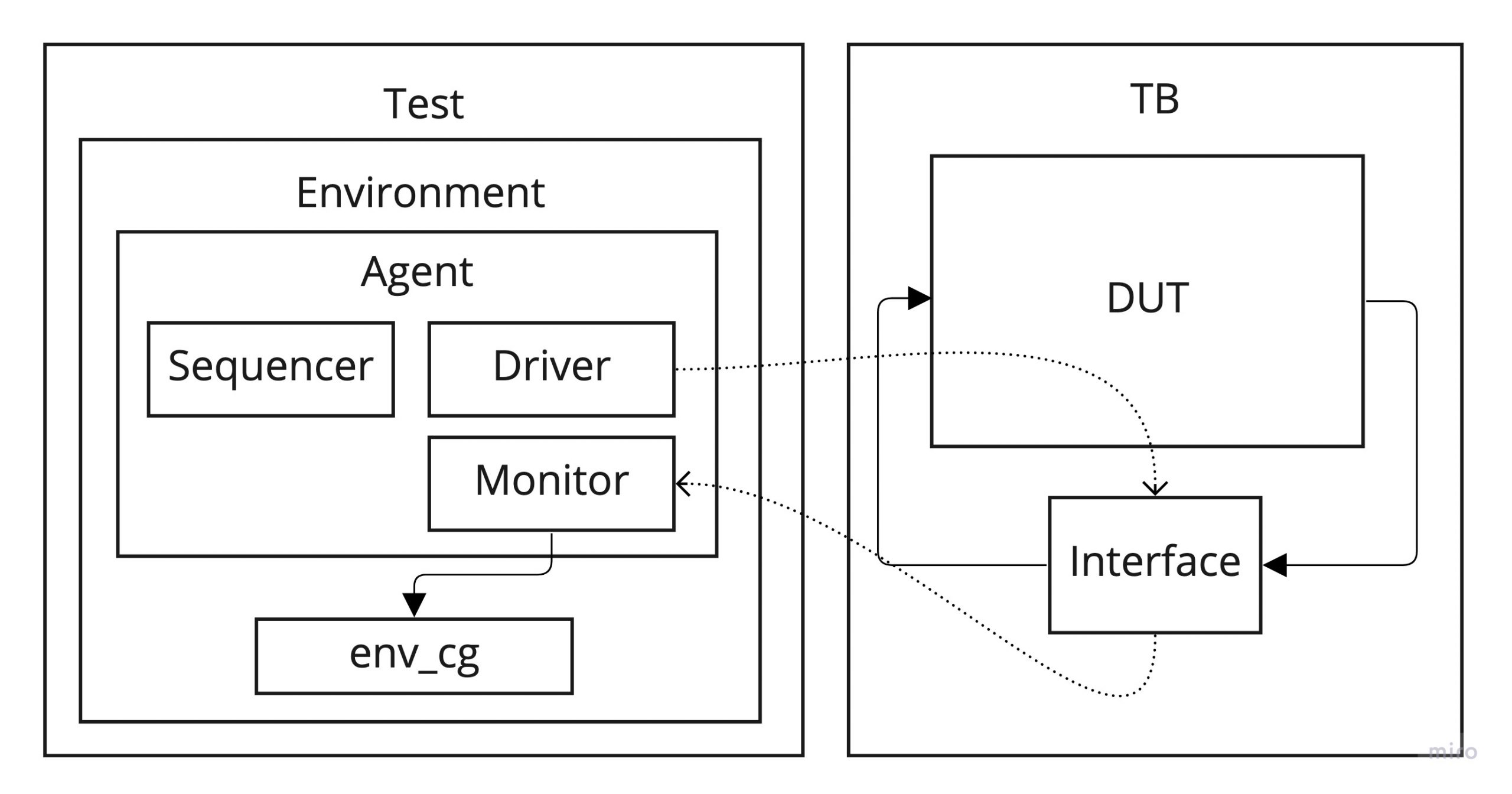
The UVM spins around the concept of abstracting the data that is sent and received from the DUT. Data abstraction allows to create and handle complex structures able to describe elaborated scenarios. For instance, we can model a burst I2C writing of 100 bytes without worrying too much about how that is going to be actually implemented. Each byte could be respresented as a transaction and from the TLM perspective we would only need to focus on the meaningful data required for fully describing the operation. Since in UVM each environment component is in charge of different actions (driving, monitoring, arbitring, etc.) a communication mechanism is required for transactions to be sent between the environment components. UVM provides TLM API and classes to do allow such communication.

In this sort of communication there is always a producer and a consumer. However, there are cases where we may want to send the transactions regardless the number of consumers (0, 1 or many). That can be implemented using analysis port and exports and is not the scope of this post.

TLM ports and exports

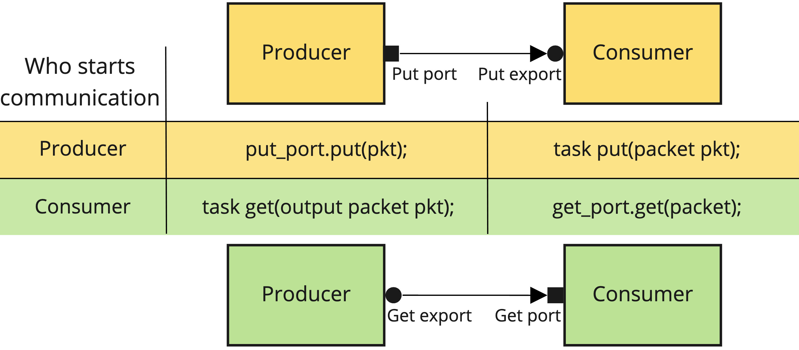
In UVM, a port class provides functions that can be called. Because of this, it will be placed on the component that initiates the communication. As we are going to see soon, the communication can be started by either the consumer or the producer, so the port class has not to be confused with the direction of the transactions.

On the other hand, an export class specifies the implementation of the functions. Therefore, it will be placed on the component that waits for the communication to be started. Again, as in the case of the port, it gives no information per se about the direction of the transactions, only gives information about who asks for them.

The TLM API implements two different ways to control the communication flow. In the case that the communication is started by the producer, then we will need to use a put port. If it is the consumer who controls the communication, then we will use a get port.

Also, an important aspect of the ports and exports is that they require always to be connected. If they remain unconnected then you will have a `uvm_error on simulation time 0 as follows:

UVM_ERROR @ 0: uvm_test_top.env.agent.put_port [Connection Error] connection count of 0 does not meet required minimum of 1

Communication started by the producer (put)

In the producer, in order to send a uvm_object, it is necessary to call the put task on the port object.

In the consumer, we need to implement the put task where we can define what we want to do with the incoming transaction. This function will be automatically called when the producer calls the port put task.

Also, there are two different types of put ports: blocking and nonblocking.

UVM TLM blocking put port

The put method implementation is a task and therefore it can consume simulation time. If we call the put method on the producer and want to wait for the consumer to finish processing it before keep executing the producer’s code, then we need a blocking put port. By waiting for the consumer to be done with the transaction sent, we can create synchronization patterns that might be useful for our verification infrastructure.

Producer

The producer calls the put() method over the put_port.

class producer extends uvm_component;

    uvm_blocking_put_port #(packet) put_port;

    `uvm_component_utils(producer)

    function new(string name="producer", uvm_component parent);
        super.new(name, parent);
        put_port = new("put_port", this);
    endfunction

    virtual task run_phase(uvm_phase phase);
        packet pkt;
        pkt = packet::type_id::create("pkt");
        if (!pkt.randomize()) `uvm_error("NO_RND", "Couldn't randomize pkt")
        put_port.put(pkt);
    endtask : run_phase
    
endclass : producer
Consumer

The consumer executes the put() task every time the producer sends a transaction. It is important to know that in the case we need to use the transaction information at a later stage, we need to clone the object so that we hold a copy of it. Otherwise, the transaction data will change as soon as the producer generates a new object since the transaction in the consumer is passed by reference. This can lead to waste an enormous amount of time debugging why the transaction information is not matching the expected values 🙂

class consumer extends uvm_component;

    uvm_blocking_put_imp #(packet, consumer) put_export;

    `uvm_component_utils(consumer)

    function new(string name = "consumer", uvm_component parent);
        super.new(name, parent);
        put_export = new("put_export", this);
    end : new

    task put(packet pkt);
        // Called everytime the producer sends a transaction
    endtask
endclass : consumer

From the code snippet above, note that the consumer who is finally going to receive the transaction uses a uvm_blocking_put_imp object. Intuitively one can think that a uvm_blocking_put_export should be used, but that’s only used in the case of having multiple layers of communication where we need to connect an export implementation with one or more intermediate layers. Please check out the section «Multiple port/export layers» for more details.

As shown above, the put_port and put_export objects are created inside the class constructor use new and not the UVM factory.

UVM TLM nonblocking put port

If we don’t want to wait for the consumer to have processed and finished the put method before continuing with the program execution in the producer, then we can use a nonblocking put port. To do so, replace in the previous producer and consumer implementation the blocking word with nonblocking when declaring the port and export.

Communication started by the consumer (get)

In the case of being the consumer who will ask for transactions, then we will need to create an export in the producer and a port in the consumer.

UVM TLM blocking get port

class producer extends uvm_component;

    uvm_blocking_get_imp #(packet, producer) get_export;
    
    `uvm_component_utils(producer)

    function new(string name="producer", uvm_component parent);
        super.new(name, parent);
        get_export = new("get_export", this);
    endfunction

    task get(output packet pkt);
        pkt = packet::type_id::create("pkt");
        if (!pkt.randomize()) `uvm_error("NO_RND", "Couldn't randomize pkt")
    endtask : get
endclass : producer
class consumer extends uvm_component;

    uvm_blocking_get_port #(packet) get_port;

    `uvm_component_utils(consumer)

    function new(string name = "consumer", uvm_component parent);
        super.new(name, parent);
        get_port = new("get_port", this);
    end : new

    virtual task run_phase(uvm_phase phase);
        Packet pkt;
        [...]
        get_port.get(pkt);
    endtask : run_phase
endclass : consumer

UVM TLM nonblocking get port

If we don’t want to wait for the producer to send the packet before continuing with the program execution in the consumer, then we can use a nonblocking get port. To do so, again, replace in previous producer and consumer implementation the blocking word with nonblocking when declaring the port and export.

Method Blocking Nonblocking
Put
Port uvm_blocking_put_port#(tr)
uvm_nonblocking_put_port#(tr)
Export uvm_blocking_put_export#(tr)
uvm_nonblocking_put_export#(tr)
Imp uvm_blocking_put_imp#(tr, parent)
uvm_nonblocking_put_imp#(tr, parent)
Get
Port uvm_blocking_get_port#(tr)
uvm_nonblocking_get_port#(tr)
Export uvm_blocking_get_export#(tr)
uvm_nonblocking_get_export#(tr)
Imp uvm_blocking_get_imp#(tr, parent)
uvm_nonblocking_get_imp#(tr, parent)

The rest of the component implementation remains the same.

Connecting ports and exports

Both port and export have to be connected together using the connect() method. This is usually done at a higher hierarchy level, i.e., the producer and/or consumer parent. For instance, in order to connect an agent’s driver with the sequencer, the connection will be done on the agent’s class on the connect_phase().

The connect() method is implemented on the port object. Therefore, the depending on the put or get method used we will need to call the connect() over the producer or the consumer. In the example below, both cases are shown. However, bear in mind that only one actually applies for connect a TLM port and export.

class pkt_agent extends uvm_agent;

    producer prod;
    consumer cons;

    `uvm_component_utils(pkt_agent)

    [...]

    virtual function void build_phase(uvm_phase phase);
        [...]
        prod = producer::type_id::create("prod", this);
        cons = consumer::type_id::create("cons", this);
    endfunction : build_phase

    virtual function void connect_phase(uvm_phase phase);
        super.connect_phase(phase);
        // Put port/export. It does not apply on get method
        prod.put_port.connect(cons.put_export);
        // Get port/export. It does not apply on put method
        cons.get_port.connect(prod.get_export);
    endfunction : connect_phase

endclass

Multiple port/export layers

In case of having multple port/export layers, such as the case depicted below, we need to connect ports with ports and exports with exports in the highest levels of hierarchy.

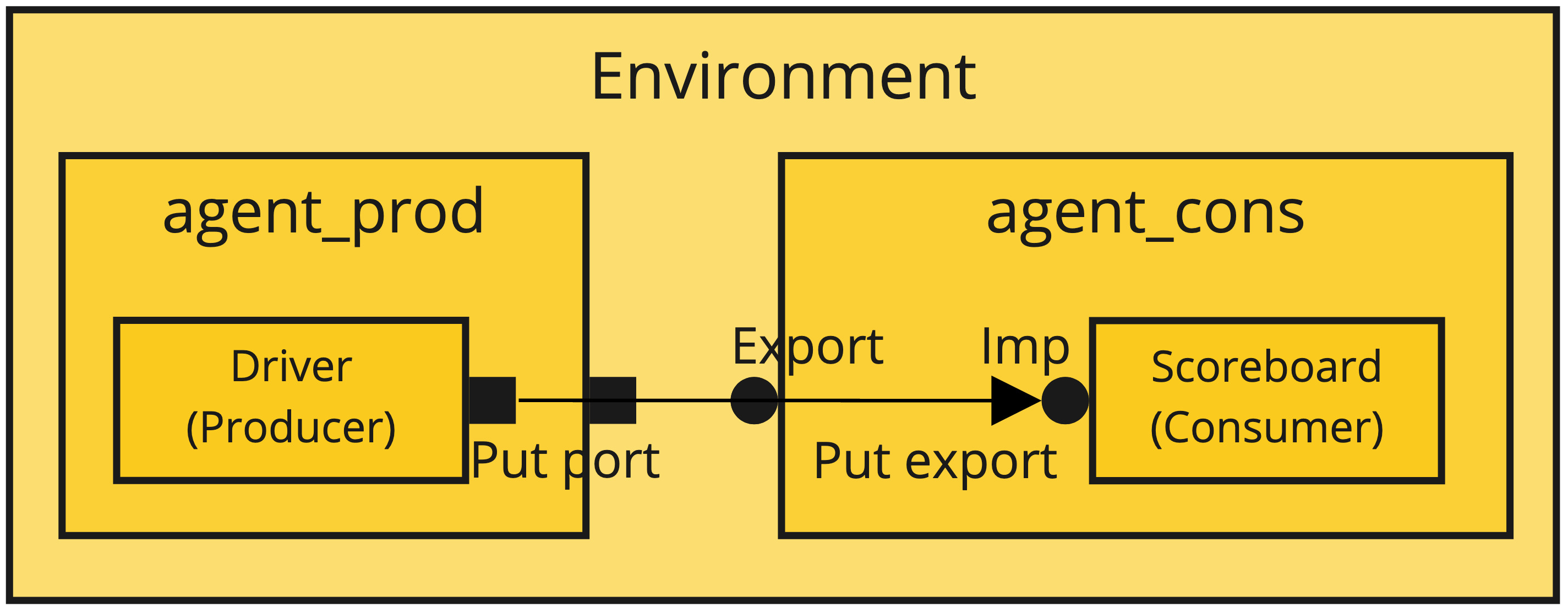
When driving the transaction outwards, we will use a port. When driving the transaction inwards AND it is not the last component, we will use an export. And finally, when driving the transaction into the last component (the destination), we will use an imp (since it is the place where we will implement the put or get method).

In this case, the connections will be done as follows:

  • Port to port: child_comp.child_port.connect(parent_port)
  • Port to export: put_port_comp.put_port.connect(export_port_comp.export_port)
  • Export to export: parent_comp.parent_port.connect(child_port.export)

An example implementating the diagram above can be:

class agent_prod extends uvm_agent;

    driver drv; // Let's assume the driver has a uvm_blocking_put_port#(packet) object
    uvm_blocking_put_port put_port;

    `uvm_component_utils(agent_prod)

    function new(string name="agent_prod", uvm_component parent);
        super.new(name, parent);
        put_port = new("put_port", this);
    endfunction

    virtual function void connect_phase(uvm_phase phase);
        super.connect_phase(phase);
        drv.put_port.connect(put_port);
    endfunction : connect_phase

endclass : agent_prod

class agent_cons extends uvm_agent;

    scoreboard scb;  // Let's assume the scoreboard has a uvm_blocking_put_imp#(packet, scoreboard) object
    uvm_blocking_put_export#(packet) put_export;

    `uvm_component_utils(agent_cons)

    function new(string name="agent_cons", uvm_component parent);
        super.new(name, parent);
        put_export = new("put_export", this);
    endfunction

    virtual function void connect_phase(uvm_phase phase);
        super.connect_phase(phase);
        put_export.connect(scb.put_export);
    endfunction : connect_phase

endclass : agent_cons

class env extends uvm_env;

    agent_prod agent_port;
    agent_cons agent_exp;

    `uvm_component_utils(env)

    function new(string name, uvm_component parent);
        super.new(name, parent);
    endfunction

    function void build_phase(uvm_phase phase);
        agent_port = agent_prod::type_id::create("agent_port", this);
        agent_exp = agent_cons::type_id::create("agent_exp", this);
    endfunction

    function void connect_phase(uvm_phase phase);
        super.connect_phase(phase);
        agent_port.put_port.connect(agent_exp.put_export);
    endfunction

endclass


In Design Verification (DV), a test is a set of stimuli that exercises the Design Under Test (DUT). The purpose of the test is to verify one or more specs and/or functionalities, so to be methodogically strict, it is absolutely mandatory for the test to contain checkers that deterministically asserts whether the design is behaving as expected or not. Otherwise, the test will not have more use than help you to prepare some nice waveforms or dangerously give you a false confidence of higher functional and code coverage.

Usually, the testcase has a fixed amount of instructions or actions to do over the DUT. This might vary slightly in the case of generating randomly the data to inject into the design, but the steps to take will be known upfront. In the case of having to fulfill some functional coverage such as covergroups, it is possible that a single run won’t be able to hit all possible scenarios that a covergroup requires to get 100% coverage. One way to overcome this is to increase the number of runs of the same test to expand the hit scenarios. However, it is not always clear how many of these are going to be required in order to reach the coverage goals. You can try increasing little by little the number of runs/seeds until you get a stable figure of coverage throughout several consecutive regressions or you can take a shortcut and increase dramatically the number of seeds. Both approaches present drawbacks however. The trial and error approach requires time which you might not have. Depending on the duration of the test and the number of runs, it may take you days to figure out what is the minimum number of tests required since each regression may take several hours. On the other hand, the «all-in» strategy may be consuming unnecessary computional resources since you might be running several orders of magnitude more tests than the ones it was actually required.

The purpose of this post is to elaborate on a way in which the functional coverage can dictate whether the test must keep trying new scenarios and in turn exercising the DUT any further or stop the simulation. This can be easily done on custom made SystemVerilog testbenches, but it is way more interesting analysing how to do this using the Universal Verification Methodology (UVM) as it is the most widely used verification framework in the semiconductor industry.

The DUT, SystemVerilog testbench and UVM environment architecture presented in this post is the simplest possible. The only purpose of them is to serve as a vehicle to illustrate the mentioned approach. Also, all the code shown in this article has been uploaded to the GitHub repo uvm-cg-driven in case you just want to dive directly into the code.

The DUT (dut.sv)

The DUT is a dummy, empty module with 3 input ports: address, data and clock. In this case study we are only interested on generating the stimuli reaching this module. Therefore, the DUT is as simple as it can be.

module dut(input [3:0] addr, data, input clk);

endmodule

The testbench (tb_sim_top.sv)

The top of the simulation just contains the instatiation of the DUT, the interface required for the UVM agent and the call for UVM to start the tests.

`include "uvm_macros.svh"
import uvm_pkg::*;
import cg_driven_pkg::*;
import pkt_agent_pkg::*;

module tb;

    dut u_dut(
        .addr(pkt_if.addr),
        .data(pkt_if.data),
        .clk (pkt_if.clk)
    );

    pkt_if pkt_if();

    initial begin
        uvm_config_db#(virtual pkt_if)::set(null, "*", "pkt_vif", pkt_if);
        run_test();
    end

endmodule : tb

UVM architecture

The only existing test is called cg_driven_test. This instantiates the cg_drive_env environment object and the sequence to be run multiple times. The environment in turn instantiates a custom-made agent called pkt_agent, which is an active agent in charge of generating random values of data, addresses and clocks. It also constains a monitor that builds transaction objects from the activity seen on the interface connected to the DUT. Finally, the transactions created at the monitor are sent through an analysis port to allow any environment component to use them.

The component that uses these transactions is instantiated directly in the environment, but there is no limitation on where it can be placed as long as it has visibility of the already mentioned monitor’s analysis port. This component, called env_cg, samples the coverage and is extended from the UVM class uvm_subscriber. In essense, the uvm_subscriber class is a component with a built-in analysis export. So we can take advantage of this and connect it with the pkt_mon analysis port. Also, we can instantiate as many covergroups as we may need. The only limitation is that a uvm_subscriber component can only receive one type of transactions using the built-in analysis export. Hence, we may want to create different uvm_subscriber for every different transaction for which we want to monitor the functional coverage.

Every time that a new transaction is sent through the analysis port by the monitor, the subscriber function write() is called, so it is a nice place to call for the covergroup sample() method.

import pkt_agent_pkg::pkt_tr;

class cg_driven_subscriber extends uvm_subscriber #(pkt_tr);

    `uvm_component_utils(cg_driven_subscriber)

    pkt_tr tr;

    covergroup cg_addr;
        c_addr : coverpoint tr.addr;
    endgroup

    function new (string name = "cg_driven_subscriber", uvm_component parent);
        super.new(name, parent);
        cg_addr = new();
    endfunction : new

    virtual function void write (pkt_tr t);
        tr = t;
        `uvm_info("SUBS", $sformatf("New transaction received. Sampling coverage"), UVM_MEDIUM)
        cg_addr.sample();
    endfunction : write

endclass : cg_driven_subscriber

We can access the covergroup information from the test through the environment object. We can create a loop that can be repeated as long as the coverpoint coverage is lower than certain value. Since every time that the sequence is executed the driver generates traffic on the interface, the monitor will be able to regenerate a transaction that will eventually reach our subscriber component. Therefore, every time that the sequence finishes, the coverpoint coverage should be updated.

class cg_driven_test extends uvm_test;

    `uvm_component_utils(cg_driven_test)

    pkt_sequence seq;
    cg_driven_env env;

    function new(string name = "cg_driven_test", uvm_component parent);
        super.new(name, parent);
    endfunction : new

    function void build_phase(uvm_phase phase);
        super.build_phase(phase);
        env = cg_driven_env::type_id::create("env", this);
    endfunction : build_phase

    virtual task main_phase(uvm_phase phase);
        super.main_phase(phase);
        phase.raise_objection(this);
        `uvm_info("TEST", "Hello, World!", UVM_LOW)
        #100ns;
        seq = pkt_sequence::type_id::create("seq");
        while(env.cg_subs.cg_addr.get_inst_coverage() < 100.0) begin
            seq.start(env.pkt_agt.sqr);
            `uvm_info("CF", $sformatf("CG coverage = %0.2f %", env.cg_subs.cg_addr.get_inst_coverage()), UVM_MEDIUM);
        end
        phase.drop_objection(this);
    endtask : main_phase

endclass : cg_driven_test

Finally, we can use the method get_inst_coverage() over the coverpoint of interest, which returns a real value with the current coverage. However, we need to be aware that depending on the simulation tool used, the coverage collection might be disabled by default. For instance, in Xcelium you need to add the switch -cov U to enable the functional coverage analysis or -cov_cgsample. Please take a look at the Makefile in the repo to see the exact switches I used.

Conclusion

This is just a simple way to use covergroups inside UVM, which provides the advantage of running just the minimum number of sequences required to fulfill the coverage goals based on one or more coverpoints. This can be very convinient since you can come up with the certainty that if the test finishes, all the targeted scenarios were visited. Of course, this can not always be used and there might be cases where the multiseed approach can boost the functional coverage much quicker. Also, it is possible that due to the nature of the covergroup and the way the stimuli is generated, the test may never reach the goal figure. Therefore, this method might be useful not only to just run the minimum necessary sequences but also to identify possible problems on the way the test is generating the transactions. All in all, it seems quite reasonable to keep this approach in mind since it can work really well on simple cases and can also provide further information on the test infrastructure capabilities.

The fixed point representation consists of the representation of decimal numbers using a binary coding scheme that can’t model exactly all decimal numbers. Before getting into details, we are going to have a brief overview on different binary encondings schemes that there are.

Binary encoding using fixed point

En the fixed point representation, the value of the represented number depends on the position of the 1’s and 0’z. For instance:
\[ (10010)_2 = 1 \cdot  2^4 + 0 \cdot 2^3 + 0 \cdot 2^2 + 1 \cdot 2^1 + 0 \cdot 2^0 = 18 \]
The dynamic range of this representation is given by the number of bits used. However, the addition operation using fixed point representation numbers is straigtforward.

Binary encoding using floating point

The number value doesn’t depend on the bit position. The binary number is split into 3 different parts: sign, mantissa and exponent

The value is computed as:

\[ \text{Value} = S \cdot M \cdot 2^{E-cte} \]

The floating point encoding provides a much greater dynamic range than the fixed point encoding. Furthermore, the resolution can be variable. Nevertheless, performing the addition operation using floating point enconding is more complex.

In order to represent integer numbers, there are two encodings that are quite used. The first one is the already mentioned fixed point encoding, whereby every bit represents a different weight of a power of 2. However, with this encoding it is not possible to represent negative numbers. To do so, the most widely used enconding is known as 2’s complement.

Fixed point encoding for unsigned integers (positive)

The encoding for N bits unsigned numbers has a range \(\left[0, 2^N -1 \right]\). In this case, the resolution is 1.

In order to compute the value of a binary number:

\[ X = \sum_{i=0}^{N-1} x_i 2^i\]

Fixed point enconding for integers with sign

The enconding for N bits numbers with sign can be done using 2’s complement. In this encoding every bit has a weight, just as in the unsigned integers. The particularity here is that the most significant bit (MSB) has a negative sign and the corresponding power of 2 weight given by its position.

\[X = -2^{-4} + 2^2 +2^0 = -11 \]

As it can be seen, the MSB has a weight of \(2^{-4}\) and a negative sign.
El 2’s complement range is \(\left[-2^{N-1}, 2^{N-1}-1 \right] \) and the resolution 1.

Comparison between numbers with sign and 2’s complement

The table illustrated the representation with and without sign and its equivalence to the decimal format. In this case, N = 3 since only 3 bits are used to represent all the numbers. The range for the representation without sign is [0, 7] whereas in the case of the representation with sign is [-4, 3].

The values that are lower than \(2^{N-1} = 2^{3-1} = 2^2 = 4\) have their direct equivalency in both encodings (blue background), i.e., both are presented as \((011)_2\)

In the case of values without sign greater than \(2^{N-1}\), they should be read as:

\[ \text{Signed} = \text{Unsigned} – 2^N \]

For instance, 6 represented as unsigned is \((110)_2\). However, \((110)_2\) interpreted as a 2’s complement number is:

\[ \text{Signed} = 6 – 2^3 = 6 – 8 = -2\]

Therefore:

\[ S = \left\{\begin{matrix}
U; & U < 2^{N-1} \\
U – 2^N ;& U \geq 2^{N-1}
\end{matrix}\right.\]

Encoding positive real numbers using fixed point

Decimal numbers can also be represented using fixed point encoding. Nonetheless, the value accuracy will depend on the number of bits used and the point position.

\[X_E = 2^{4} + 2^2 +2^0 = 21 \]
\[X_Q = 2^{2} + 2^0 +2^{-2} = 5.25 \]

The position of the point is imaginary since it not specified internally in any way. From the position of the point towards the left, the numbers represent positive powers of 2. Towards the right, negative powers of 2. The resolution of this enconding is given by the LSB.
\[ X =  \left(\sum_{i=0}^{N-1} x_i 2^i  \right) \cdot 2^{-b} \]

The notation used to describe this enconding is \([N, b]\), where \(N\) is the total number of bits and \(b\) is the number of fractional bits. For example, \([6,3]\) means 6 bits in total 3 of which are fractional. In this case, the resolution is \(2^{-3} = 0.125\).

Enconding real numbers using fixed point in 2’s complement

When representing real numbers with sign using 2’s complement, the range of the numbers is \([-2^{N-1}\cdot Q, (2^{N-1}-1) \cdot Q]\), where N is the total number of bits and Q the resolution, which is \(Q = 2^{-b}\).

\[ X = \left(-x_{N-1} 2^{N-1} + \sum_{i=0}^{N-2} x_i 2^i  \right) \cdot 2^{-b} \]

  • Example 1:
    • N = 6, b = 3, format [6,3].
    • Range: \(\left[2^{6-1}\cdot 2^{-3}, (2^{6-1}-1)\cdot 2^{-3} \right] = \left[-4, 3.875\right] \).
    • Resolution: \(2^{-3} = 0.125\).
  • Example 2:
    • N = 5, b = 2, format [5,2].
    • Range: \(\left[2^{5-1}\cdot 2^{-2}, (2^{5-1}-1)\cdot 2^{-2} \right] = \left[-4, 3.75\right] \).
    • Resolution: \(2^{-2} = 0.25\)

Encoding dynamic range

The dynamic range of an encoding is determined by the amount of numbers used to encode a range of number. For instance, in the fixed point encoding without sign, the range is \([0, \left(2^{N}-1\right)\cdot Q]\) and the resolution \(Q=2^{-b}\).

The dynamic range is the relationship between the maximum encoding difference \([-2^{N-1}, 2^{N-1} 1]\) and the encoding resolution.

\[ DR = \frac{N_{max}-N_{min}}{Q} = \frac{ \left(2^{N}-1\right)-0}{Q} = 2^{N}-1 \]

In the case of the 2’s complement encoding, the range is \([-2^{N-1}, 2^{N-1}-1]\) and the resolution is again \(Q= 2^{-b}\). The dynamic range is also \(2^{N}-1\).

If this is computed in dB, defining the dynamic range as \(20\log_{10}\{·\}\), we can obtain that the dynamic range is approximately 6.02N dB. Therefore, every bit increase the encoding dynamic range in 6.02 dB.

Effects of the finite accuracy

The factor of working with encodings with finite accuracy it has effects on the signal we are working with. The effects can be of two different types:

  • Decrease the number of integer bits, which reduces the range of the encoding. This can lead to misrepresent the signal using a particular encoding. For example, a sine with range [0, 8] can’t be encoded with U[4, 3] since numbers greater than \(2^{4} \cdot 2^{-3} = 2\) can’t be represented. This can have two different consequences over the signal:
    • Wrap: the signal is wrapped and the higher numbers are represented near the low values of the range.

Example: S[4,3], range [-1, 0.875], resolution \(2^{-3} = 0.125\). If this encoding represent a number out of the range, \(1.125 = (01.001)_2 \), we only have 1 bit to represent the integer part. Therefore, it will be cut to \((1.001)_2\) which converting this 2’s complement number to decimal it is \( \left(-2^{3} + 2^{0} \right) \cdot 2^{-3} = -0.875\)

    • Clamp: all numbers outside the range are «saturated» to the maximum (or minimum) value. In order to represent the campling, it is necessary to include extra logic to take these cases into account.

  • Quantization: since all decimal numbers can’t be represented due to the finite accuracy of the encoding, all possible values will be multiples of the resolution. Every real number between two multiples of the resolution will be mapped to one of the nearest multiples. Therefore, the signal will look like a stair wave. Depending the mapping technique used (nearest, floor, ceil, etc.) the effects are different. From the frequency point of view, the quantization adds white noise that is spreaded througout all the signal band (from 0 Hz to half of the sampling frequency \(\frac{f_s}{2}\).
    • Floor: «flooring» means to round to the nearest low value. This produces a maximum error of -Q and in average -Q/2. However, computationally is simple to resolve.

    • Nearest: round to the nearest value. It rounds up if Q/2 is exceeded and down if the value is below Q/2.

Implementation of nearest and floor

In MATLAB the functions round() and floor() can be used for computing the nearest and floor integer value of a number. Therefore, if we want to round to 2 decimals the number 12.5432 what we need to do is:

  • Shift two digits to the left multiplying the number by 100: 12.5432 · 100 = 1254.32
  • Apply the rounding method: floor(1254.32) = 1254
  • Shift two digits to the right dividing the number by 100: 1254/100 = 12.54

In the binary encoding, the operation is the same. The only difference is that instead of using powers of 10 to shift number, we use powers of 2.

Example: round to 3 fractional bits \(1.28515625 = (01.01001001)_2 \)

  • Shift 3 digits to the left multiplying by \(2^3\): \(1.28515625 \cdot 2^3 = 10.28125\)
  • Apply the floor() function. floor(10.28125) = 10
  • Shift 3 digits to the right multiplying by \(2^{-3}\): \(10 \cdot 2^{-3} = 1.25 = (01.010)_2\)

Quantizing fixed point number in MATLAB

In MATLAB we can use the function quatize(q, a). It can be used to compute the quantized number with a given fixed point encoding. This function has two parameters:

  • q: is the quantizer object that defines the enconding to be used. It is defined with the function quantizer(Format, Mode, Roundmode, Overflowmode), where:
    • Format: [N b]
    • Mode: ‘fixed’ o ‘ufixed’ for a fixed point encoding signed or unsigned.
    • Roundmode: ‘floor’, ‘round’ for nearest.
    • Overflowmode: ‘saturate’ or ‘wrap’
  • a: number to quantify

Definition of fixed point in Simulink

In Simulink, we can use the function fixdt(Signed, WordLength, FractionLength) to the define the encoding format.

Modifying the resolution or scaling

Extending the resolution

This is the situation in which we want to represent the fractional part with more bits than in the original encoding. This operation is as straightforward padding with zeros at the right of the binary number.

Reducing the resolution

The fractional part of the number is represented with less bits than in the original encoding. Therefore, the resolution is shrinked.

Example:

\(A = 2.625 = (010.101)_2\)

\(A [6,3] \rightarrow A =  A_e \cdot 2^{-3} =(010101)_2 ~~A_e = (010101)_2 21 \)

\(A’ [4,1] \rightarrow A’ =  A’_e \cdot 2^{-2} =(0101)_2~~A’_e = (0101)_2 = 5 \)

This operation can be intuitively understood as changing the integer part of the number. For instance, the initial number could be interpreted as unsigned as \(A_e = 21\) because the integer part was using 6 bits in total. If we cut the total number of bits used to 4, then the unsigned value is lower than before (5). FInally, if we need to scale the number moving the «fixed point» where necessary to obtain the final value on the new encoding.

Example:

\(A’_e = floor\left(A_e \cdot 2^{-2}\right) = 5\)

In this case, we need to multiply by \(2^{-2}\) because we need to go from a resolution of \(2^{-3}\) to \(2^{-1}\). Therefore, we need to shift the point 2 positions to the right.

The uvm_object class is the base class for all UVM classes. From it, all the rest of classes are extended. It provides basic functionalities such as print, compare, copy and similar methods.

This class can be used when defining reusable parts of a sequence items. For example, in a packet like uvm_sequence_item, we could define a uvm_object extended object for defining the header. This would be:

class packet_header extends uvm_object;

   rand bit [2:0] len;
   rand bit [2:0] addr;

   `uvm_object_utils_begin(packet_header)
      `uvm_field_int(len, UVM_DEFAULT)
      `uvm_field_int(addr, UVM_DEFAULT)
   `uvm_object_utils_end

   function new (string name="packet_header");
      super.new(name);
   endfunction : new

endclass : packet_header

This packet_header could be included in a packet class for conforming the uvm_sequence_item (the transaction) which will compose the sequences:

class simple_packet extends uvm_sequence_item;

   rand packet_header header;
   rand bit [4:0] payload;

   `uvm_object_utils_begin(simple_packet)
      `uvm_field_object(header, UVM_DEFAULT)
      `uvm_field_int(payload, UVM_DEFAULT)
   `uvm_object_utils_end

   function new (string name = "simple_packet");
      super.new(name);
      header = packet_header::type_id::create("header");
   endfunction : new

endclass : packet


Let’s z be a 2D point in the space as \(z = x + jy\), if we want to rotate this point a given angle \(\theta\), we get the following expressions:
\[e^{j\theta} \cdot z = \left(\cos{\theta} + j \sin{\theta}\right)\left(x+jy\right) \\ = x\cos{\theta}-y\sin{\theta} + j \left(y \cos{\theta} + x \sin{\theta} \right) \\ = x’ + j y’ \]

Then, for a generic point, the rotation can be expressed as an equation system, where \(x’\) and \(y’\) are the new coordinates, \(\theta\) is the rotation angle and \(x\) and \(y\) are the original coordinates:
\[\begin{bmatrix}
x’\\
y’
\end{bmatrix}=
\begin{bmatrix}
\cos{\theta} & -\sin{\theta}\\
\sin{\theta} & \cos{\theta}
\end{bmatrix}\begin{bmatrix}
x\\
y
\end{bmatrix} \]

This rotation can be coded in MATLAB as:


%% Function to rotate vector
function v = rotate(P, theta)
    rot = [cos(theta) -sin(theta);
           sin(theta) cos(theta)];
    v = rot*P;
end

A possible implementation of the cordic algorithm could be:


%% Clear all previous values
clear all;

%% Define vectors
A = [2;-3];
O = [0;0];

%% Define accuracy
error_limit = 0.01;

%% Initialize variables
start_angle = pi/2; % 90º
current_angle = start_angle;
acc_angle = 0;

A_rotated = A;
steps = 0;

% Second quadrant (90º - 180º)
if(A_rotated(1) < 0 && A_rotated(2) > 0)
    A_rotated = rotate(A_rotated, -pi/2);
    acc_angle = pi/2;
% Third quadrant (180º - 270º)
elseif(A_rotated(1) < 0 && A_rotated(2) < 0)
    A_rotated = rotate(A_rotated, -pi);
    acc_angle = pi;
% Forth quadrant (270º - 360º)
elseif(A_rotated(1) > 0 && A_rotated(2) < 0)
    A_rotated = rotate(A_rotated, -3*pi/2);
    acc_angle = 3*pi/2;    
end


%% Compute angle
% Keep rotating while error is too high
while(abs(A_rotated(2)) > error_limit)
    % Represent current vector
    quiver(0, 0,A_rotated(1), A_rotated(2));
    % Keep previous vectors
    hold on;
    % Decrease angle rotation
    current_angle = current_angle/2;
    % (For debugging purposes)
    current_angle_deg = current_angle*180/pi;
    % Save current error
    error = A_rotated(2);
    % If y coordinate is still positive
    if(error > 0)
        % Rotate again conterclockwise
        A_rotated = rotate(A_rotated, -1*current_angle);
        % Accumulate rotated angle
        acc_angle = acc_angle + current_angle;
    % If y coordinate is negative
    else
        % Rotate vector clockwise
        A_rotated = rotate(A_rotated, current_angle);
        % Substract current angle to the accumulator because we have
        % overcome the actual angle value
        acc_angle = acc_angle - current_angle;
    end
    
    % (For debugging purposes)
    acc_angle_deg = acc_angle*180/pi;
    % Increase step counter
    steps = steps + 1;
end

% Print angle, hypotenuse length and number of steps needed to compute
fprintf('Angle = %f\nHypotenuse = %f\nNumber of steps: %d\n', acc_angle*180/pi, A_rotated(1), steps);


%% Function to rotate vector
function v = rotate(P, theta)
    rot = [cos(theta) -sin(theta);
           sin(theta) cos(theta)];
    v = rot*P;
end


I have coded an interactive applet to illustrate the algorithm. It has been done using the p5.js library. The error limit has been set to \(0.5\).

#define round(x) x >= 0.0 ? (int)(x + 0.5) : ((x - (double)(int)x) >= -0.5 ? (int)x : (int)(x - 0.5))

Example:

#include <stdio.h>

#define round(x) x >= 0.0 ? (int)(x + 0.5) : ((x - (double)(int)x) >= -0.5 ? (int)x : (int)(x - 0.5))

void main(void){
   float f1 = 3.14, f2 = 6.5, f3 = 7.99;
   int r1, r2, r3;
   r1 = round(f1);
   r2 = round(f2);
   r3 = round(f3);


   printf("r1 = %d\nr2 = %d\nr3 = %d\n", r1, r2, r3);
}

The console output is:

r1 = 3
r2 = 7
r3 = 8

UVM introduces the concept of phases to ensure that all objects are properly configured and connected before starting the runtime simulation. Phases contribute to a better synchronised simulation and enable to the verification engineer to get better modularity of the testbench.

UVM phases consists of:

  1. build
  2. connect
  3. end_of_elaboration
  4. start_of_simulation
  5. run
    1. reset
    2. configure
    3. main
    4. shutdown
  6. extract
  7. check
  8. report
  9. final

The run phase has been simplified to get a better picture of how phases worked. Nevertheless, all subphases in the run phase have a pre_ and post_ phase to add flexibility. Therefore, the run phase is actually composed by the following phases:

  1. run
    1. pre_reset
    2. reset
    3. post_reset
    4. pre_configure
    5. configure
    6. post_configure
    7. pre_main
    8. main
    9. post_main
    10. pre_shutdown
    11. shutdown
    12. post_shutdown

Although all phases play an important role, the most relevant phases are:

  • build_phase: objects are created
  • connect_phase: interconnection between objects are hooked
  • run_phase: the test starts. The run_phase is the only phase which is a task instead of a function, and therefore is the only one that can consume time in the simulation.

UVM phases are executed from a hierarchical point of view from top to down fashion. This means that the first object that executes a phase is the top object, usually

testbench  test  environment agent {monitor, driver, sequencer, etc}

Nevertheless, in the connect phase, this happens the other way round in a down to top fashion.

{monitor, driver, sequencer} agent environment test testbench

To use UVM in your Verilog test bench, you need to compile the UVM package top. To do so, you need to include it on your file by using:

`include "uvm_macros.svh"
import uvm_pkg::*;

The uvm_pkg is contained in the uvm_pkg.sv that must be passed to the compiler. Therefore, it is necessary to indicate the UVM path to the compiler. In Cadence Incisive Enterprise Simulator (IES) is as easy as to specify -uvm switch.

In Modelsim, from Modelsim console, run:

vsim -work work +incdir+/path/to/uvm-1.1d/src +define+UVM_CMDLINE_NO_DPI +define+UVM_REGEX_NO_DPI +define+UVM_NO_DPI

After compilation, click on Simulate > Start simulation and select the tb in the work library. Then, run the simulation for the desired time.

When an operation such as an addtion or a substraction is done using different size operands than final variable, it is necessary to extend sign to ensure the operation is done properly.

Example:

logic signed [21:0] acc;
logic signed [5:0] data_in;
logic [3:0] offset;

Wrong:

acc = data_in + offset;

Sign on data_in will not be respected. data_in will be filled with 0 before doing the operation and won’t be taken as negative (if applies).

Correct:

acc = {{16{data_in[5]}},data_in} + offset;

Extend sign to match number of acc_add bits before doing operation