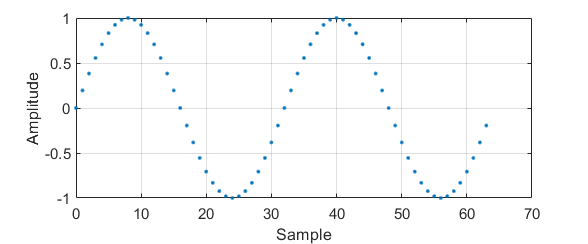
DFT can be thought as a simple change of basis. In the time domain, every sample of a signal represents its amplitude at that very instant.
\[ y\left[n\right] = \sin{\left( \frac{2\pi k }{N} n\right)} \]
Nevertheless, when applying a transformation such as the DFT, every sample means something different.
The DFT is computed as the scalar product between the signal and a orthogonal base. This base is as follows:
\[ \{\boldsymbol{w}^{(k)}\}_{\{k=0,1,…,N-1\}} \]
\[ w_n = e^{j \frac{2\pi}{N}nk}\]
If some of these base vectors are plotted with the imaginary part in the Y axe and the real part in the X axe:
DFT calculation
The DFT of a signal can be computed then, applying a change of basis over the desired signal.
\[ X\left[k\right] = \sum_{n=0}^{N-1} x\left[n\right] e^{-j\frac{2\pi}{N}nk}, \text{ } k = 0,1,…,N-1 \]
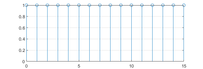
DFT of a \(\delta\left[n\right]\)
\[ x\left[n\right] = \delta[n] = \left\{\begin{matrix}
1 & n = 0\\
0 & otherwise
\end{matrix}\right. \]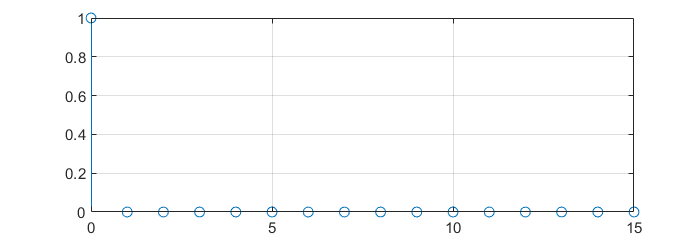 \[X\left[k\right] = \sum_{n=0}^{N-1}{\delta\left[n\right] e^{-j\frac{2\pi}{N}nk}}\]
\[ X\left[k\right] = 1 \cdot e^{-j\frac{2\pi}{N}\cdot 0 \cdot k} = 1 \]
 DFT of a cosine
\[ x\left[n\right] = 4 \cos{\left(\frac{2\pi}{4}n\right)} = 4 \cos{\left(\frac{2\pi 4}{16}n\right)} = \frac{4}{2} \left[e^{ \frac{2\pi}{16} 4n} + e^{-j \frac{2\pi}{16} 4n} \right]\]
[To be finished]