Coordinates, orthogonal coordinates and BJT transistors in CircuiTikZ

The LaTeX package CircuiTikZ is an excelent way to draw circuits in a standard and elegant manner. However, it can get quite tricky when you need to specify the absolute coordinates of all the nodes of your schematic.

In order to facilitate this process coordinates and orthogonal coordinates come to the rescue.

Coordinates

You can provide a name for every node in your circuit. For instance, in the following line:

\draw (0,0) -- (2,0) coordinate(pointA);

point (2,0) can be accessed from now on using (pointA):

\draw (0,0) -- (2,0) coordinate(pointA);
\draw (pointA) to[R] ++(2,0);

The resistor will be placed from pointA, i.e., (2,0), to (4,0). Remember that the operator ++() makes a relative movement with respect the previous point (in this case (2,0)) and «stores» the position so that any new component in the same \draw statement will start from that point, i.e., (4,0). Also, +() makes the relative movement with respect the original point without storing the new position and not affecting any subsequent element in the \draw statement.

When using hardcoded coordinates like in previous example it might not be very powerful per se, but at least it may help to understand the way the diagram is written.

However, they can solve a lot of headaches when you need to draw two or more components in parallel.

Orthogonal coordinates

In case you want to align to different nodes, orthogonal coordinates computes automatically the X and Y of the new node.

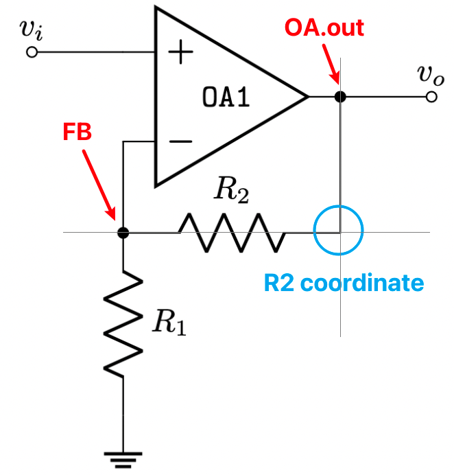
From CircuiTikZ manual, section 2.2, where a classic non-inverting amplifier using an op amp is being drawn:

\draw (FB) to[R=$R_2$] (FB -| OA.out) -- (OA.out)

The way the previous line can be read is:

1. From the coordinate FB, add a resistor to
2. The horizontal value of FB (that’s why - is next to FB) and the veritical of OA.out (that’s why | is before OA.out)
3. Then draw a line from this previous point to the op amp output OA.out

Example

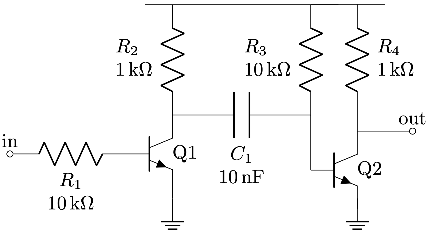
Below you will find an example where all previous concepts are applied in order to draw the schematic of a basic pulse generator with BJT’s.

\usepackage[american]{circuitikz}
\usepackage{siunitx}

\begin{circuitikz} []
   \draw (0,0) node[bjtnpn] (Q1){Q1};
   \draw (Q1.B) to[R, l2={$R_1$ and \SI{10}{\kilo\ohm}}, l2 halign =c] ++(-2,0) to[short,-o] ++(-0.1, 0) node[above]{in};
   \draw (Q1.C) to[R, l2={$R_2$ and \SI{1}{\kilo\ohm}}] ++(0, 2) coordinate(R2t);
   \draw (Q1.E) to[short] ++(0, -0.1) coordinate(Q1gnd) node[ground] (GND){} ;
   \draw (Q1.C) to[C, l2_=$C_1$ and \SI{10}{\nano\farad}, l2 halign =c] ++(2.5,0) coordinate(c1n) to[short] +(0,-1) node[bjtnpn, anchor=B](Q2){Q2};
   \draw (c1n) to[R,l2=$R_3$ and \SI{10}{\kilo\ohm}] ++(0,2) coordinate (R3t);
   \draw (R2t) -- (R3t);
   \draw (R2t) -- +(-0.5,0);
   \draw (R3t) -- +(0.5, 0);
   \draw (Q2.E) -- (Q2.E |- Q1gnd) node[ground]{};
   \draw (Q2.C) -- (Q2.C |- c1n) coordinate(R4b) to[R,l2_=$R_4$ and \SI{1}{\kilo\ohm}] (Q2.C |- R2t) coordinate(R4t) -- (R3t);
   \draw (R4t) -- ++(0.5,0);
   \draw (Q2.C) to[short, -o] ++(1,0) node[above]{out};
\end{circuitikz}