Introduction

Any two-terminal network whose internal circuitry is made up solely of resistors, current sources and voltage sources can be simplified to a voltage source (\(V_{TH}\)) with a resistor in series (\(R_{TH}\)). This is called Thevenin’s theorem.

In order the find the Thevenin’s equivalent circuit, it is necessary to follow two steps:

  1. Find \(R_{th}\) by turning off all internal sources and connecting an external current source.
  2. Find \(V_{th}\) by turning on all internal sources and leaving the external current source in open circuit.

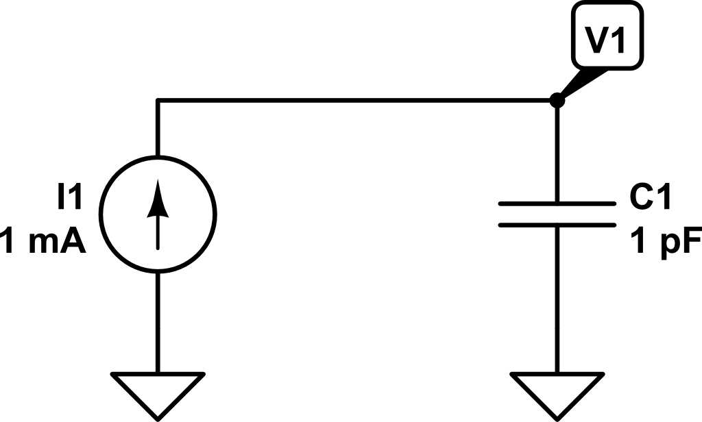
When we turn off all internal supply sources we set \(v_{int} = 0\), i.e., shorting the internal voltage supply sources, and we set \(i_{int} = 0\), i.e., opening the internal current supply sources. Then, we apply an external current supply source (\(I_{ext}\)) and compute the correspondent voltage between the two terminals (\(V_{1}\)). The value of \(R_{TH}\) will be:
\[
R_{th} = \frac{V_1}{I_{ext}}
\]

On the second step, we will turn on again all the internal sources and set the external current source as open circuit. The voltage seen at the two terminals of interest will be \(V_{th}\)

Example

We will start the circuit analysis by setting all internal supply sources off. All the voltage sources will be shorted whereas the current sources will be left in open circuit.

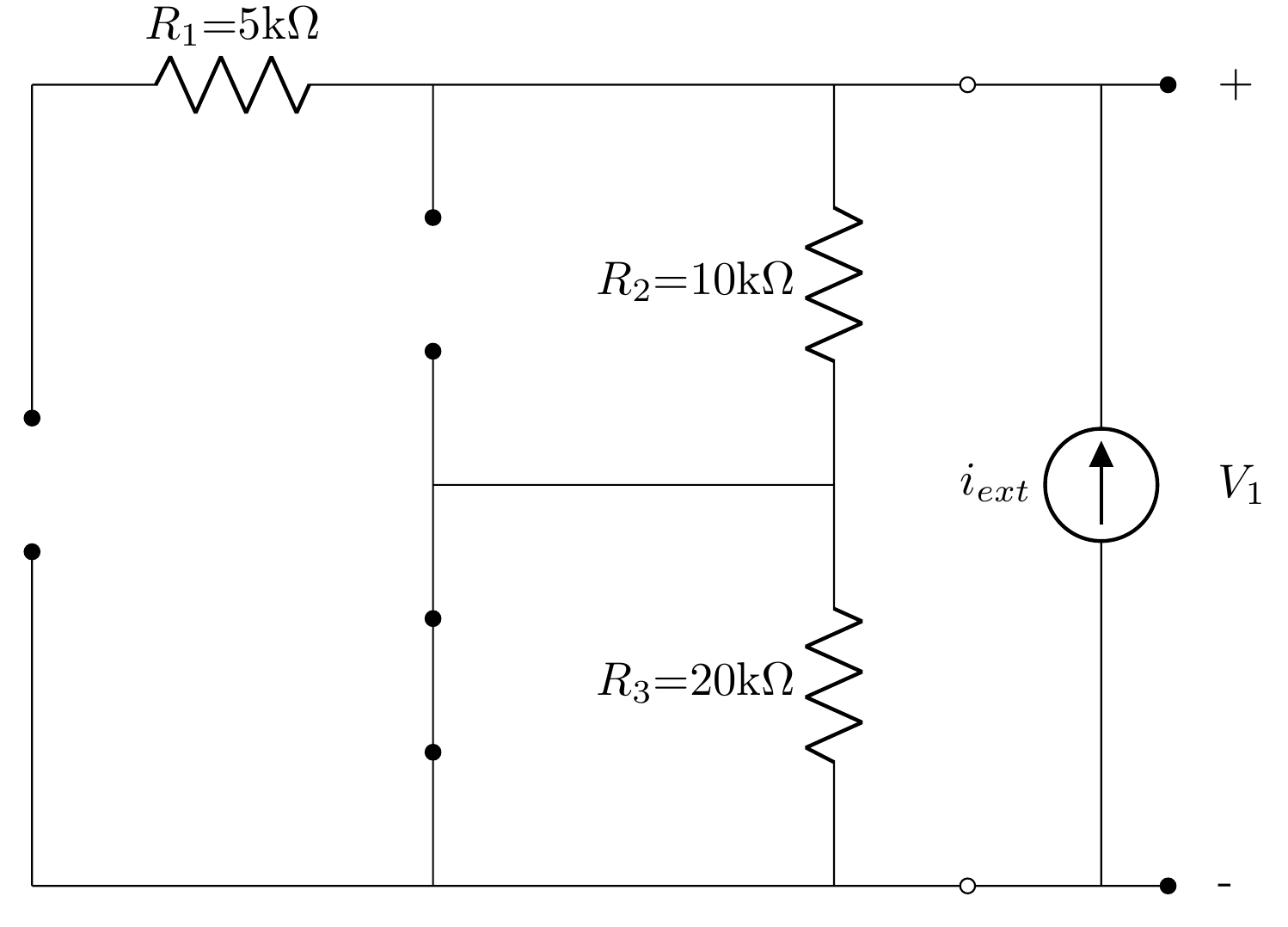
From here, now we are going to compute what is the voltage \(V_{1}\).

Since there is no path to the negative terminal on \(R_1\) and \(R_3\) is shorted, they don’t contribute to the output voltage \(V_1\).

Instead, \(V_1\) can be computed as:
\[
V_1 = i_{ext} \cdot R_2
\]

Therefore, the Thevenin’s resistance is:
\[
R_{TH} = \frac{V_1}{i_{ext}} = \frac{i_{ext} \cdot R_2}{i_{ext}} = R_2
\]

Now we need to compute Thevenin’s voltage \(V_{TH}\). For this we are going to turn on again all the internal sources, i.e., leaving the circuit as it originally was, and computing the voltage across its two terminals.

If we apply the Kirchhoff’s current law (KCL) on every node:

\[
I_2 + i_3 = i_5
\]

\[
I_1 = i_3
\]

\[
i_5 = I_2 + i_4 + i_6
\]

From Equation 1, we find that

\[
i_1 + i_3 = \frac{V_{TH} – V_3}{R_2} \Rightarrow \left(i_1 + i_3\right) R_2 + V_3 = V_{TH}
\]

\[
V_{TH} = \left(0.5~mA + 1~{mA}\right) \cdot 10~{k}\Omega + 10~{V} = 25~V
\]

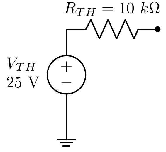
With this information, we can say that an equivalent circuit seen from these two terminals can be:

A capacitor is an electronic device able to store electrical energy in an electrical field. Usually, the capacitor is defined in its most simple version as a device with two plates with area \(A\), separated by air (or any other dielectric material) a distance \(d\).

Parallel plate capacitor.svg
By inductiveload – own drawing, done in Inkscape 0.44, Public Domain, Link

If a current source is forced through the capacitor, the electrons (charge) will be deposited in one of the plates, creating in turn a electrical field across them. There won’t be any effective charge transference from one plate to the other because the space between them is filled with a dielectric material (non conductive). However, the electrical field across it can force the repulsion or attraction of charge at the other side of the plate.

Capacitor schematic with dielectric.svg
By Papa November – self-made SVG version of Image:Dielectric.png, incorporating Image:Capacitor schematic.svg as its base., CC BY-SA 3.0, Link

A capacitor is characterized by its capacitance. The capacitance is measured in Farads (F) and defines the ratio between the amount of charge needed to increase one volt at the terminals of the capacitor.

\[ C= \frac{Q}{V} \]

Therefore, a capacitor with 1 F will need 1 Coulomb (1 C) of charge to set 1 V across its terminals. Remember, that 1 C represents the amount of energy transported by a constant current of 1 A in 1 second.

Behavior of a capacitor connected to a DC current source

Let’s see what happens when we connect a DC current source to a capacitor. Transforming a little bit the previous expression, we can obtain:

\[ C = \frac{Q}{V}  \Rightarrow V = \frac{Q}{C} \]

As \(Q = \int{i\left(t\right) dt}\), we can get the voltage across the capacitor as a function of the time and the current:

\[ V\left(t\right) = \frac{1}{C} \int{i\left(t\right) dt} \]

Therefore, if we inject a constant current of \(1~mA\) for \(1~ns\), the voltage \(V_1\left(t\right)\) will be as follows:

In this example, what would be the charge stored in the capacitor at time \(t_1 = 1~ns\)?

\[ C = Q/V \Rightarrow Q = C \cdot V = 1~pF ·  1V = 1\cdot10^{-12}~C \]

Now, what would be the value of the voltage \(V_1\) if at time \(t_1 = 1~ns\) a second capacitor \(C_2\) (discharged) of \(2~pF\) of capacitance is connected?

At that very moment in which the second capacitor is connected in parallel, the charge in \(C_1\) will be distributed between \(C_1\) and \(C_2\).

The effective capacitance now is \(3~pF\) (\(1~pF  + 2~pF\)). Remember that using the capacitance definition, we got:

\[ V = \frac{Q}{C_p} = \frac{Q}{C_1 + C_2} = \frac{1\cdot 10^{-12} C}{1\cdot10^{-12}~F + 2\cdot10^{-12}~F} = 0.333~V \]

Therefore, as the capacitance now has increased and the charge remains the same (although shared between \(C_1\) and \(C_2\)), according to the previous expression the voltage has to drop.

If we would like to know the charge stored in every individual capacitor at time \(t_1 = 1~ns\), we could compute it as:
\[ Q = C \cdot V\]
\[ Q_1\left(t_1 = 1~ns\right) = C_1 \cdot V_1\left(t_1 = 1~ns\right) = 1~pF \cdot 0.333~V = 3.33\cdot10^{-13}~C\]
\[ Q_2\left(t_1 = 1~ns\right) = C_2 \cdot V_1\left(t_1 = 1~ns\right) = 2~pF \cdot 0.333~V = 6.66\cdot10^{-13}~C\]

The result is consistent with the previous calculation stating that the amount of charge at \(t_1=1~ns\) was \(Q = 10^{-12}~C\).

Finally, let’s see what happens if at time \(t_2 = 2~ns\) the capacitor \(C_2\) is again disconnected and only capacitor \(C_1\) is connected to the current source.

At time \(t_2 = 2~ns\) the voltage \(V_1\) will have increased to:

\[V\left(t_2 = 2~ns\right) = V_1\left(t_{1}^{+}\right) + \frac{1}{C_1 + C_2} \int_{t_1 = 1~ns}^{t_2 = 2~ns}{i\left(t\right) dt} \]

\[V\left(t_2 = 2~ns\right) = 0.333 V + \frac{1}{1~pF + 2~pF} \int_{t_1 = 1~ns}^{t_2 = 2~ns}{1~mA~dt} = 0.333~V +0.333~V = 0.666~V\]

Now the charge will be distributed as follows:

\[ Q_1\left(t_2 = 2~ns\right) = C_1 \cdot V_1\left(t_1 = 2~ns\right) = 1~pF \cdot 0.666~V  = 6.66\cdot10^{-13}~C\]
\[ Q_2\left(t_2 = 2~ns\right) = C_2 \cdot V_1\left(t_1 = 2~ns\right) = 2~pF \cdot 0.666~V = 1.22\cdot10^{-12}~C\]

If \(C_2\) is disconnected, the charge stored in it will be lost and won’t be redistributed towards \(C_1\). Therefore, the total amount of charge in the system at \(t_2 = 2~ns\) will only be that on \(C_1\).

Now, the voltage increment at the same rate as in the period \(0 < t < t_1 = 1~ns\).

Therefore, if we plot the voltage from \(t=0~ns\) to \(t_3 = 3~ns\), we would get the following voltage profile for \(V_1\):

The uvm_object class is the base class for all UVM classes. From it, all the rest of classes are extended. It provides basic functionalities such as print, compare, copy and similar methods.

This class can be used when defining reusable parts of a sequence items. For example, in a packet like uvm_sequence_item, we could define a uvm_object extended object for defining the header. This would be:

class packet_header extends uvm_object;

   rand bit [2:0] len;
   rand bit [2:0] addr;

   `uvm_object_utils_begin(packet_header)
      `uvm_field_int(len, UVM_DEFAULT)
      `uvm_field_int(addr, UVM_DEFAULT)
   `uvm_object_utils_end

   function new (string name="packet_header");
      super.new(name);
   endfunction : new

endclass : packet_header

This packet_header could be included in a packet class for conforming the uvm_sequence_item (the transaction) which will compose the sequences:

class simple_packet extends uvm_sequence_item;

   rand packet_header header;
   rand bit [4:0] payload;

   `uvm_object_utils_begin(simple_packet)
      `uvm_field_object(header, UVM_DEFAULT)
      `uvm_field_int(payload, UVM_DEFAULT)
   `uvm_object_utils_end

   function new (string name = "simple_packet");
      super.new(name);
      header = packet_header::type_id::create("header");
   endfunction : new

endclass : packet


\[ s_k = (k\cdot A) \bmod B\]

\(s_k\) is the pseudo-random number and \(A\) and \(B\) are prime numbers. \(k\) is in the range \([0,B-1]\). If \(k\) is greater than \(B-1\), the results will be repeat as \(B\) is the period of the sequence.
For example, \(A = 7\) and \(B = 17\). This sequence written in MATLAB could be:

A = 7;
B = 17;
n = [];

t = 0:B;
for i=0:B
    n = [n mod(i*A,B)];
end

stem(t,n);


Pseudo-random values
Periodicity of the sequence when k > B

Let’s z be a 2D point in the space as \(z = x + jy\), if we want to rotate this point a given angle \(\theta\), we get the following expressions:
\[e^{j\theta} \cdot z = \left(\cos{\theta} + j \sin{\theta}\right)\left(x+jy\right) \\ = x\cos{\theta}-y\sin{\theta} + j \left(y \cos{\theta} + x \sin{\theta} \right) \\ = x’ + j y’ \]

Then, for a generic point, the rotation can be expressed as an equation system, where \(x’\) and \(y’\) are the new coordinates, \(\theta\) is the rotation angle and \(x\) and \(y\) are the original coordinates:
\[\begin{bmatrix}
x’\\
y’
\end{bmatrix}=
\begin{bmatrix}
\cos{\theta} & -\sin{\theta}\\
\sin{\theta} & \cos{\theta}
\end{bmatrix}\begin{bmatrix}
x\\
y
\end{bmatrix} \]

This rotation can be coded in MATLAB as:


%% Function to rotate vector
function v = rotate(P, theta)
    rot = [cos(theta) -sin(theta);
           sin(theta) cos(theta)];
    v = rot*P;
end

A possible implementation of the cordic algorithm could be:


%% Clear all previous values
clear all;

%% Define vectors
A = [2;-3];
O = [0;0];

%% Define accuracy
error_limit = 0.01;

%% Initialize variables
start_angle = pi/2; % 90º
current_angle = start_angle;
acc_angle = 0;

A_rotated = A;
steps = 0;

% Second quadrant (90º - 180º)
if(A_rotated(1) < 0 && A_rotated(2) > 0)
    A_rotated = rotate(A_rotated, -pi/2);
    acc_angle = pi/2;
% Third quadrant (180º - 270º)
elseif(A_rotated(1) < 0 && A_rotated(2) < 0)
    A_rotated = rotate(A_rotated, -pi);
    acc_angle = pi;
% Forth quadrant (270º - 360º)
elseif(A_rotated(1) > 0 && A_rotated(2) < 0)
    A_rotated = rotate(A_rotated, -3*pi/2);
    acc_angle = 3*pi/2;    
end


%% Compute angle
% Keep rotating while error is too high
while(abs(A_rotated(2)) > error_limit)
    % Represent current vector
    quiver(0, 0,A_rotated(1), A_rotated(2));
    % Keep previous vectors
    hold on;
    % Decrease angle rotation
    current_angle = current_angle/2;
    % (For debugging purposes)
    current_angle_deg = current_angle*180/pi;
    % Save current error
    error = A_rotated(2);
    % If y coordinate is still positive
    if(error > 0)
        % Rotate again conterclockwise
        A_rotated = rotate(A_rotated, -1*current_angle);
        % Accumulate rotated angle
        acc_angle = acc_angle + current_angle;
    % If y coordinate is negative
    else
        % Rotate vector clockwise
        A_rotated = rotate(A_rotated, current_angle);
        % Substract current angle to the accumulator because we have
        % overcome the actual angle value
        acc_angle = acc_angle - current_angle;
    end
    
    % (For debugging purposes)
    acc_angle_deg = acc_angle*180/pi;
    % Increase step counter
    steps = steps + 1;
end

% Print angle, hypotenuse length and number of steps needed to compute
fprintf('Angle = %f\nHypotenuse = %f\nNumber of steps: %d\n', acc_angle*180/pi, A_rotated(1), steps);


%% Function to rotate vector
function v = rotate(P, theta)
    rot = [cos(theta) -sin(theta);
           sin(theta) cos(theta)];
    v = rot*P;
end


I have coded an interactive applet to illustrate the algorithm. It has been done using the p5.js library. The error limit has been set to \(0.5\).

    1. Open http://dl.altera.com/?edition=lite
    2. Login and click on desired Quartus version download
    3. Click in the individual file links to start download (Akamai DLM3 Download Manager might not work).
    4. Extract Quartus installer.
    5. Run setup.sh: ./setup.sh
    6. Select desired devices.
    7. For launching modelsim, install libxft2 32 bit version library: sudo apt install libxft2:i386. Then execute ./vsim in the path intelFPGA_lite/17.1/modelsim_ase/linuxaloem/
#define round(x) x >= 0.0 ? (int)(x + 0.5) : ((x - (double)(int)x) >= -0.5 ? (int)x : (int)(x - 0.5))

Example:

#include <stdio.h>

#define round(x) x >= 0.0 ? (int)(x + 0.5) : ((x - (double)(int)x) >= -0.5 ? (int)x : (int)(x - 0.5))

void main(void){
   float f1 = 3.14, f2 = 6.5, f3 = 7.99;
   int r1, r2, r3;
   r1 = round(f1);
   r2 = round(f2);
   r3 = round(f3);


   printf("r1 = %d\nr2 = %d\nr3 = %d\n", r1, r2, r3);
}

The console output is:

r1 = 3
r2 = 7
r3 = 8

UVM introduces the concept of phases to ensure that all objects are properly configured and connected before starting the runtime simulation. Phases contribute to a better synchronised simulation and enable to the verification engineer to get better modularity of the testbench.

UVM phases consists of:

  1. build
  2. connect
  3. end_of_elaboration
  4. start_of_simulation
  5. run
    1. reset
    2. configure
    3. main
    4. shutdown
  6. extract
  7. check
  8. report
  9. final

The run phase has been simplified to get a better picture of how phases worked. Nevertheless, all subphases in the run phase have a pre_ and post_ phase to add flexibility. Therefore, the run phase is actually composed by the following phases:

  1. run
    1. pre_reset
    2. reset
    3. post_reset
    4. pre_configure
    5. configure
    6. post_configure
    7. pre_main
    8. main
    9. post_main
    10. pre_shutdown
    11. shutdown
    12. post_shutdown

Although all phases play an important role, the most relevant phases are:

  • build_phase: objects are created
  • connect_phase: interconnection between objects are hooked
  • run_phase: the test starts. The run_phase is the only phase which is a task instead of a function, and therefore is the only one that can consume time in the simulation.

UVM phases are executed from a hierarchical point of view from top to down fashion. This means that the first object that executes a phase is the top object, usually

testbench  test  environment agent {monitor, driver, sequencer, etc}

Nevertheless, in the connect phase, this happens the other way round in a down to top fashion.

{monitor, driver, sequencer} agent environment test testbench

To use UVM in your Verilog test bench, you need to compile the UVM package top. To do so, you need to include it on your file by using:

`include "uvm_macros.svh"
import uvm_pkg::*;

The uvm_pkg is contained in the uvm_pkg.sv that must be passed to the compiler. Therefore, it is necessary to indicate the UVM path to the compiler. In Cadence Incisive Enterprise Simulator (IES) is as easy as to specify -uvm switch.

In Modelsim, from Modelsim console, run:

vsim -work work +incdir+/path/to/uvm-1.1d/src +define+UVM_CMDLINE_NO_DPI +define+UVM_REGEX_NO_DPI +define+UVM_NO_DPI

After compilation, click on Simulate > Start simulation and select the tb in the work library. Then, run the simulation for the desired time.